by Matthew Barsalou, guest blogger
In the 1935 book The Design of Experiments, Ronald A. Fisher used the example of a lady tasting tea to demonstrate basic principles of statistical experiments. In Fisher’s example, a lady made the claim that she could taste whether milk or tea was poured first into her cup, so Fisher did what any good statistician would do—he performed an experiment.
The lady in question was given eight random combinations of cups of tea with either the tea poured first or the milk poured first. She was required to divide the cups into two groups based on whether the milk or tea was poured in first. Fisher’s presentation of the experiment was not about the tasting of tea; rather, it was a method to explain the proper use of statistical methods.
Understanding how to properly perform a statistical experiment is critical, whether you're using a data analysis tool such as Minitab Statistical Software or performing the calculations by hand.
The Experiment
A poorly performed experiment can do worse than just provide bad data; it could lead to misleading statistical results and incorrect conclusions. A variation on Fisher’s experiment could be used for illustrating how to properly perform a statistical experiment. Statistical experiments require more than just an understanding of statistics. An experimenter must also know how to plan and carry out an experiment.
A possible variation on Fisher’s original experiment could be performed using a man tasting coffee made with or without the addition of sugar. The objective is not actually to determine if the hypothetical test subject could indeed determine if there is sugar in the coffee, but to present the statistical experiment in a way that is both practical and easy to understand. Having decided half of the cups of coffee would be prepared with sugar and half would be prepared without sugar, the next step is to determine the required sample size. The formula for sample size when using a proportion is

In this equation the n is the sample size, p is the probability something will occur and q is the probability it will not occur. Z is the Z score for the selected confidence level and E is the margin of error. We use 0.50 for both p and q because there will be a 50/50 chance of randomly selecting the correct cup. The Z score is based on the alpha (α) level we select for the confidence level; in this case we choose an alpha of 0.05, so that there is a 5% chance of failing to reject the null hypothesis when it should actually be rejected. We will use 15% for E. This means the sample size would be:

We can’t perform 0.68 tests, so we round up to the next even whole number, which would mean 44 trials. We would need 22 cups of coffee with sugar and 22 cups of coffee without sugar. That is a lot of coffee so the cup size will be 10 ml each. There is a risk that different pots of coffee will not be the same as each other due to differences such as the amount of coffee grain used or the cooling of the coffee over time. To counter this, the experimenter would brew one large pot of coffee and then separate it into two containers; one container would receive the sugar.
A table is then created to plan the experiment and record the results. The first 22 samples would contain sugar and the next 22 would not. Simply providing the test subject with the cups in the order they are listed would risk the subject realizing the sugar is in the first half so randomization will be required to ensure the test subject is unaware of which cups contain sugar. Fisher in The Design of Experiments referred to randomization as an “essential safeguard.” A random sequence generator can used to assign the run order to the samples.
The accuracy of the results could be increased by using blinding. The experimenter may subconsciously give the test subject signals that could indicate the actual condition of the coffee. This could be avoided by having the cups of coffee delivered by a second person who is unaware of the status of the cups. The use of blinding adds an additional layer of protection to the experiment.
The Analysis (by Hand)
Suppose the test subject correctly identified 38 out of 44 samples, which results in a proportion of 0.86. This could have been the result of random chance and not actually correctly identifying the samples so a one sample proportion test could be used to evaluate the results. A one sample proportion test has several requirements that must be met:
- The sample size times the probability of an occurrence must be greater than or equal to 5 so: np ≥5. We have 44 samples and the chance of a random occurrence is 0.5 so 44 x 0.5 = 22.
- The sample size times the probability something will not occur must be greater than or equal to 5 so: nq ≥ 5. We have 44 samples and the chance of an occurrence not occurring is 0.5 so 44 x 0.5 = 22.
- The sample size must be large; generally, there should be 30 or more samples.
All requirements have been met so we can use the one sample hypothesis test to analyze the results. The test statistic is:

The P represents the actual proportion and P0 represents the hypothesized proportion of the results if they had been random.
We need a null hypothesis and an alternative hypothesis to valuate. The null hypothesis states that nothing happened so P = P0. The alternative could be the two values are not equal; however, this could lead to rejecting the null hypothesis if the gentlemen tasting the coffee guessed incorrectly more often than should have happened through chance alone. So we would use P > P0, which means we are using a one-tailed upper-tail hypothesis test. The resulting hypothesis test would be:
Null Hypothesis (H0): P = P0
Alternative Hypothesis (Ha): P > P0
We want a 95% confidence level so we check a Z score table and determi ne the proper Z score to use is 1.96. The null hypothesis would be rejected if the calculated Z value is higher than 1.96. The formula is:

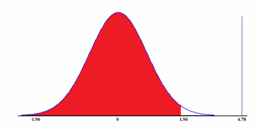
The resulting Z score is greater than 1.96 so we reject the null hypothesis. The rejection region for this test is the red area of the distribution depicted in figure 1. Had the resulting Z score been less than 1.96, we would have failed to reject the null hypothesis when using an α of 0.05.

The Analysis (Using Statistical Software)
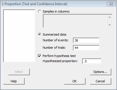
We can also perform this analysis using statistical software. In Minitab, select Stat > Basic Statistics > 1 Proporortion... and fill out the dialog box as shown below:

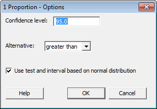
Then click on the "Options" button to select "greater than" as the alternative hypothesis, and check the box that tells the software to use the normal distribution in its calculations:

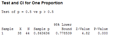
Minitab gives the following output:

The z-value of 4.82 differs slightly from our hand-calculated value since Minitab used more decimals than we did, but the practical result is the same: the z-value is greater that 1.96, so we reject the null hypothesis. Minitab also gives us a p-value, which in this case is 0. And as a wise statistician once said, "If the P-value's low, the null must go."
It is important to note that rejecting the null hypothesis does not automatically mean we accept the alternative hypothesis. Accepting the alternative hypothesis is a strong conclusion; we can only conclude there is insufficient evidence to reject it when compared against the null hypothesis and the null hypothesis only used as a comparison with the alternative hypothesis. Fisher himself, in The Design of Experiments, tells us “the null hypothesis is never proved or established, but is possibly disproved, in the course of experimentation.”
Fisher’s Results
As for the original experiment, Fisher’s son-in-law the statistician George E.P. Box informs us in the Journal of the American Statistical Association the lady in question was Dr. Muriel Bristol and her future husband reported she got almost all choices correct. In The Lady Tasting Tea David Salsburg also confirms the lady in question could indeed taste the difference; he was so informed by Professor Hugh Smith, who was present while the lady tasted her tea.
Fisher never actually reported the results; however, what mattered in Fisher’s tale is not whether or not somebody could taste a difference in a drink, but using the proper methodology when performing a statistical experiment.


