Boxers or briefs.
Republican or Democrat.
Yin or yang.
Why is it that life often seems to boil down to two choices?
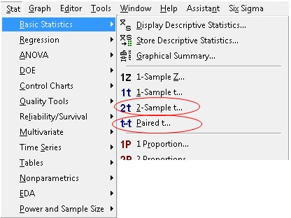
Heck, it even happens when you open the Basic Stats menu in Minitab. You’ll see a choice between a 2-sample t-test and a paired t-test:

Which test should you choose? And what’s at stake?
Ask a statistician, and you might get this response: "Elementary, my dear Watson. Choose the 2-sample t-test to test the difference in two means: H0: µ1 – µ2 = 0 Choose the paired t-test to test the mean of pairwise differences H0: µd = 0."
You gaze at your two sets of data values, mystified. Do you have to master the Greek alphabet to choose the right test?
όχι !
(That's Greek for “no”)
Base Your Decision on How the Data Is Collected
Dependent samples: If you collect two measurements on each item, each person, or each experimental unit, then each pair of observations is closely related, or matched.
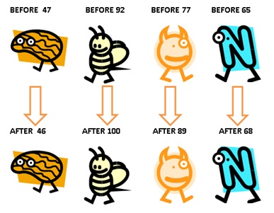
For example, suppose you test the computer skills of participants before and after they complete a computer training course. That produces a set of paired observations (Before and After test scores) for each participant.

In that case, you should use the paired t-test to test the mean difference between these dependent observations. (See the orange guy at left shaped like a lopsided peanut? That’s me. Training failed to improve my computer graphics skills. Hence the cheesy 1990s ClipArt).
Paired observations can also arise when you measure two different items subject to the same unique condition.
For example, suppose you measure tread wear on two different types of bike tires by putting both tires on the same bicycle. Then each bike is ridden by a different rider. To compare 20 pairs of tires, you use 20 different bicycles/riders.
Because each bicycle is ridden different distances in different conditions, measuring the tread wear for the two tires on each bike produces a set of paired (dependent) measurements. To account for the unique conditions that each bike was subject to, you’d use a paired t-test to evaluate the differences in mean tread wear.
Independent samples: If you randomly sample each set of items separately, under different conditions, the samples are independent. The measurements in one sample have no bearing on the measurements in the other sample.
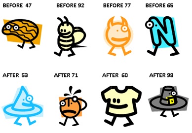
Suppose you randomly sample two different groups of people and test their computer skills. You take one random sample from people who have not taken a computer training course and record their test scores. You take a second random sample from another group of people who have completed the computer training course and record their test scores.

Because the two samples are independent, you must use the 2-sample t test to compare the difference in the means.
If you use the paired t test for these data, Minitab assumes that the before and after scores are paired: The 47 score before training is associated with a 53 score after training. A 92 score before training is associated with a 71 score after training, etc.
You could end up pairing Mark Zuckerberg’s Before test score with Lloyd Christmas’ After test score.
Invalid pairings like that can lead to very erroneous conclusions.
Paired vs 2-Sample Designs
If you’re planning your study and haven’t collected data yet, be aware of the possible ramifications of using 2-sample vs a paired design. The difference in the designs could drastically affect the amount of data you'll need to collect.
For example, suppose you design your study to measure the test scores of the same 15 participants before and after they complete a computer training course. The paired t-test test gives the following results:
Paired T-Test and CI: Before, After
Paired T for Before - After
N Mean StDev SE Mean
Before 15 97.07 26.88 6.94
After 15 101.60 27.16 7.01
Difference 15 -4.533 3.720 0.960
95% CI for mean difference: (-6.593, -2.473)
T-Test of mean difference = 0 (vs not = 0): T-Value = -4.72 P-Value = 0.000
Because the p-value (0.000) is less than alpha (0.05), you conclude that the mean difference between the Before and After test scores is statistically significant.
Now suppose instead you had designed a study to collect two independent samples: 1) the test scores from 15 people who had not completed computer training (Before) and 2) the tests scores from 15 different people who had completed the computer training (After).
For the sake of argument let's suppose you wind up with the same exact data values for the Before and After scores that you did with the paired design. Here's what you obtain when you analyze the data using the 2-sample t test.
Two-Sample T-Test and CI: Before, After
Two-sample T for Before vs After
N Mean StDev SE Mean
Before 15 97.1 26.9 6.9
After 15 101.6 27.2 7.0
Difference = mu (Before) - mu (After)
Estimate for difference: -4.53
95% CI for difference: (-24.78, 15.71)
T-Test of difference = 0 (vs not =): T-Value = -0.46 P-Value = 0.650 DF = 27
The sample size, the standard deviation, and the estimated difference between the means are exactly the same for both tests. But note the whopping difference in p-values—0.000 for the paired t-test and 0.650 for the 2-sample t-test.
Even though the 2-sample design required twice as many subjects (30) as the paired design (15), you can’t conclude there’s a statistically significant difference between the means of the Before and After test scores.
What’s going on? Why the huge disparity in results?
A Paired Design Reduces Experimental Error
By accounting for the variability caused by different items, subjects, or conditions, and thereby reducing experimental error, the paired design tends to increase the signal-to-noise ratio that determines statistical significance. This can result in a more efficient design that requires less resources to detect a significant difference, if one exists.
Because 2-sample design doesn’t control for the variability of the experimental unit, a much larger sample is needed to achieve statistical significance for a given difference and variability in the data, as shown below:
Two-Sample T-Test and CI: Before, After
Two-sample T for Before vs After
N Mean StDev SE Mean
Before 270 97.1 26.0 1.6
After 270 101.6 26.3 1.6
Difference = mu (Before) - mu (After)
Estimate for difference: -4.53|
95% CI for difference: (-8.95, -0.11)
T-Test of difference = 0 (vs not =): T-Value = -2.01 P-Value = 0.045 DF = 537
Remember, these are independent samples. So this translates to 270 + 270 = 540 subjects for the study—compared to only 15 subjects in the paired design!
That gain in efficiency comes from controlling for person-to-person variability -- a good thing to do because that variability is not a primary objective of this study. It's a nuisance factor, something that creates “extraneous noise” that gets in the way of “hearing” the main effect that you're most interested in.
So next time you’re planning T for 2, give it a hard think.
If it’s possible to satisfy your objectives using a paired t design rather than a 2-sample t design, you may be wise to do so.
Note: Click here to download the Minitab project file with the sample data used in these examples.


