


A t-test is one of the most frequently used procedures in statistics.
But even people who frequently use t-tests often don’t know exactly what happens when their data are wheeled away and operated upon behind the curtain using statistical software like Minitab.
It’s worth taking a quick peek behind that curtain.
Because if you know how a t-test works, you can understand what your results really mean. You can also better grasp why your study did (or didn’t) achieve “statistical significance.”
In fact, if you’ve ever tried to communicate with a distracted teenager, you already have experience with the basic principles behind a t-test.
Anatomy of a t-test
A t-test is commonly used to determine whether the mean of a population significantly differs from a specific value (called the hypothesized mean) or from the mean of another population.
For example, a 1-sample t-test could test whether the mean waiting time for all patients in a medical clinic is greater than a target wait time of, say, 15 minutes, based on a random sample of patients.
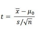
 To determine whether the difference is statistically significant, the t-test calculates a t-value. (The p-value is obtained directly from this t-value.) To find the formula for the t-value, choose Help > Methods and Formulas in Minitab, then click Basic statistics > 1-sample t > Test statistic. Here's what you'll see:
That jumble of letters and symbols may look like an incantation from a sorcerer’s book.
But the formula is much less mystical if you remember there are two driving forces behind it: the numerator (top of the fraction) and the denominator (bottom of the fraction).
The Numerator Is the Signal
The numerator in the 1-sample t-test formula measures the strength of the signal: the difference between the mean of your sample (xbar) and the hypothesized mean of the population (µ0).
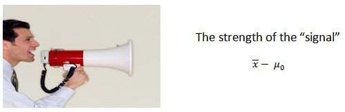
Consider the patient waiting time example, with the hypothesized mean wait time of 15 minutes.
If the patients in your random sample had a mean wait time of 15.1 minutes, the signal is 15.1-15 = 0.1 minutes. The difference is relatively small, so the signal in the numerator is weak.
However, if patients in your random sample had a mean wait time of 68 minutes, the difference is much larger: 68 - 15 = 53 minutes. So the signal is stronger.
The Denominator is the Noise
The denominator in the 1-sample t-test formula measures the variation or “noise” in your sample data.

S is the standard deviation—which tells you how much your data bounce around. If one patient waits 50 minutes, another 12 minutes, another 0.5 minutes, another 175 minutes, and so on, that’s a lot of variation. Which means a higher s value—and more noise. If, on the other hand, one patient waits 14 minutes, another 16 minutes, another 12 minutes, that’s less variation, which means a lower value of s, and less noise.
What about the √n (below the s)? That’s the square root of your sample size. What that does, very loosely speaking, is “average” out the variation based on the number of data values in the sample. So, all things being equal, a given amount of variation is “noisier” for a smaller sample than for a larger one.
The t-Value: The Ratio of Signal to Noise
As the above formula shows, the t-value simply compares the strength of the signal (the difference) to the amount of noise (the variation) in the data.
If the signal is weak relative to the noise, the (absolute) size of the t-value will be smaller. So the difference is not likely to be statistically significant:
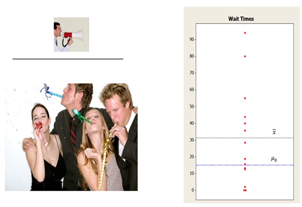
On the graph at right, the difference between the sample mean (xbar) and the hypothesized mean (µ0) is about 16 minutes. But because the data is so spread out, this difference is not statistically significant. Why? The t-value—the ratio of signal to noise—is relatively small due to the large denominator.
However, if the signal is strong relative to the noise, the (absolute) size of the t-value will be larger. So the difference between xbar and the µ0 is more likely to be statistically significant:
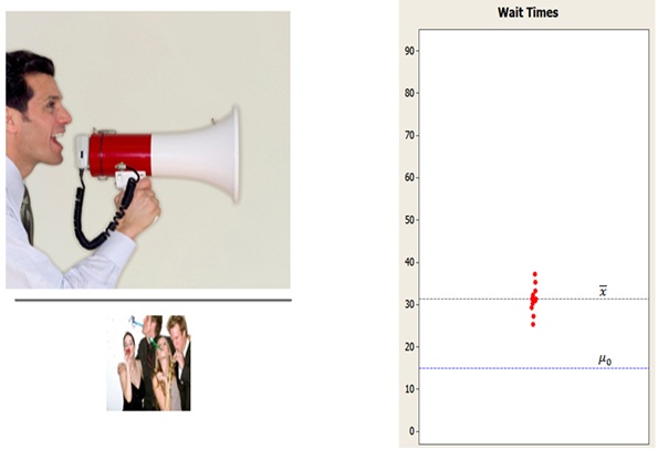
On this graph, the difference between the sample mean (xbar) and the hypothesized mean (µ0) is the same as on the previous graph—about 16 minutes. The sample size is also the same. But this time, the data is much more tightly clustered. Due to less variation, the same difference of 16 minutes is now statistically significant!
Statistically Significant Messages
So how is the t-test like telling a teenager to clean up the mess in the kitchen?
If the teenager is listening to music, playing a video game, texting friends, or distracted by any of the other umpteen sources of "noise" that pervade our lives, the louder and stronger you need to make your verbal signal to achieve "significance." Alternatively, you could insist on removing those sources of extraneous noise before you communicate—in which case you wouldn't need to raise your voice at all.
Similarly, if your t-test results don't achieve statistical significance, it could be for any of the following reasons:
- The difference (signal) isn't large enough. Nothing you can do about that, assuming that your study is properly designed and you've collected a representative sample.
- The variation (noise) is too great. This is why it's important to remove or account for extraneous sources of variation when you plan your analysis. For example, you could use a control chart to identify and eliminate sources of special-cause variation from your process before you collect data for a t-test on the process mean.
- The sample is too small. Remember the effect of variation is lessened by sample size. That means for a given difference and a given amount of variation, a larger sample is more likely to achieve statistical significance, as shown in this graph:
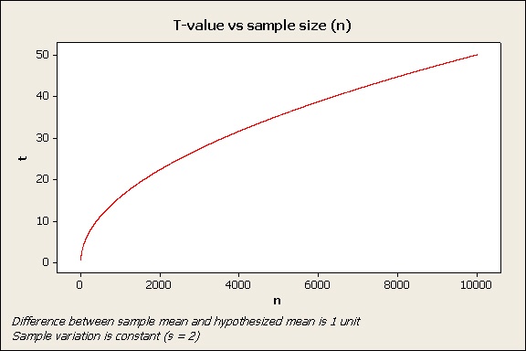
(This effect also explains why an extremely large sample can produce statistically significant results even when a difference is very small and has no practical consequence.)
By the way, in case you're wondering, these basic relationships are similar for a 2-sample t-test and a paired t- test. Although their formulas are a bit more complex (see Help > Methods and Formulas> Statistics> Basic Statistics), the basic driving forces behind them are essentially the same.
These formulas also explain why statisticians often cringe in response to the language sometimes used to convey t-test results. For example, a statistically insignificant t-test result is often reported by stating, “There is no significant difference...”
Literally speaking, it ain't necessarily so.
There may actually be a significant difference. But because your sample was too small, or because extraneous variation in your study was not properly accounted for, your study wasn't able to demonstrate statistical significance. You're on safer ground saying something like "Our study did not find evidence of a statistically significant difference."
Now, if you're still with me, you might be asking, but why is it called a t-test? And where does the p-value come from? You haven't explained any of that!
Sorry…I’m out of space and time. I’ll talk about those concepts in an upcoming post.
[no response]
JOHNNY, I SAID, I'LL TALK ABOUT THOSE CONCEPTS IN AN UPCOMING POST!!!!
Note: To find out more about how the p-values are calculated for a t-test, see this follow-up post.