How the taste of wine is described often reads like a poem: “full-bodied and rich but not heavy, high in alcohol, yet neither acidic nor tannic, with substantial black cherry flavor despite its delicacy...” Flowers and fruits are commonly used as descriptors, meant to help drinkers understand the flavors in a glass of wine. This poetry reflects that some consider the conversion of fruit to wine be an art form.
Yet flavor all comes down to chemical compounds that impact the taste of your wine. Behind the loving descriptions of wine as living art, there’s science. And statistical regression can help.
What Flavors a Wine?
Of course, wine shares many of the natural chemical compounds found in fruit and spices, so its understandable to use those as descriptors. Specific chemical compounds will consistently inform our tasting experience of what is sweet, sour or bitter, for example.
Then there are the essentials of good wine, for which there are no substitutes: good grapes of good quality, diligent wine making practices and barrel aging. Each of the winemaking phases will have a different impact on flavor.
Flavor changes occur due to different chemicals being present in the wine due to occurrences in these stages of the process. All the flavors in wine come from the grapes and the winemaking process, of course, but manipulating these phases can result in a wine that has a better flavor.
Wine tasting may sound ethereal but flavor all comes to chemical compounds, that impact the taste of your wine. Behind the loving descriptions of wine as living art, there’s science. Acids primarily add sour notes. Alcohol compounds also affect taste. Ethanol adds bitter, sweet, and sour flavors etc…. If one wants to be able to use knowledge of the impact of certain compounds on flavor, they must understand which phase will naturally produce that compound.
Identifying a Good Wine From a Bad Wine
It is unavoidable that wine tastes vary from person to person and that there are many different profiles of wine tasters (De Gustibus non est disputandum: “In matters of taste, there can be no disputes”), however we know that some wines are obviously better than others, and most people would probably recognize a good wine from a bad one.
When you need to understand situations like this in which variability and noise play an important part, statistical models are very efficient at identifying the key inputs out of seemingly completely chaotic data.
This article details how wine-tasting data and powerful modeling techniques yielded insight into variables that were important to a panel of experienced wine-tasters.
The analysis illustrates that even taste preferences, can be assessed with statistics if you choose the right analysis.
We are interested in using statistics to understand whether a wine that has, for instance, more sulphates or more chlorides would taste better. Based on that understanding, it could be possible to make a better wine. We will consider many potential predictors, such as acidity, sulphur dioxide, and percentage of alcohol.
This article has been updated to demonstrate the new version of Minitab Statistical Software. Want to try Minitab 19 for yourself? Download a 30-day free trial.
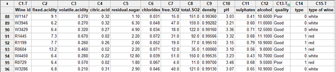
The Taste Test
A panel of oenologists tasted several types of white and red wines and provided binary assessments of quality—good (1) or poor (0)—for each. Our goal is to identify which of these many variables have a significant effect on wine quality.
Using Regression to Analyze Binary Taste Data
Simple graphs are not sufficient to identify which variables might be important due to complexity and variability in this data set. Regression analysis lets us see how multiple factors affect an outcome, so it is an ideal method to look at the wine-tasting variables.
However, our panel simply ranked each wine as either high- or low-quality. This means we have binary and not continuous response data, so we need to proceed with caution — using a standard regression or ANOVA to analyze a binary response is generally not a good idea.
Because binary data follow a binomial distribution rather than a normal, bell-shaped distribution, standard regression may result in probability predictions that are negative or larger than 100%. We might get an unnecessarily complex model, in which some spurious interactions seem to be significant. In addition, the variance for binary data is not constant.
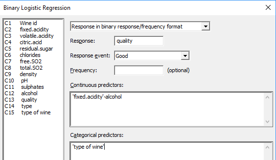
Fortunately, there’s a simple solution, since we have binary response data, we simply need to use the appropriate tool for this: binary logistic regression.
Full Model Regression Analysis
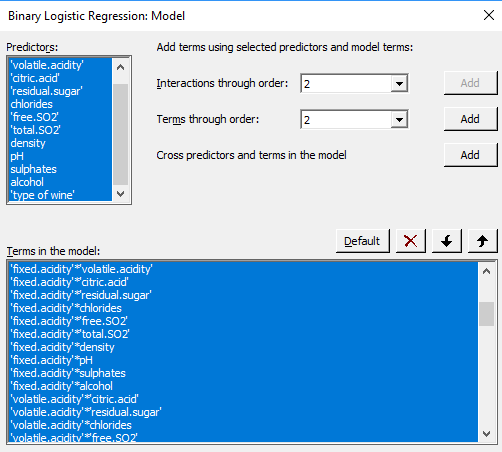
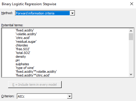
A standard practice in regression analysis is to start with the “full model,” one that includes all of the potentially significant factors for which you collected data. In this case, we begin the analysis by including all variables and all interactions between those variables and types of wine.
To include interactions, in Minitab go to Stat > Regression > Binary Logistic Regression > Fit Binary Logistic Model > Model > Add interactions.
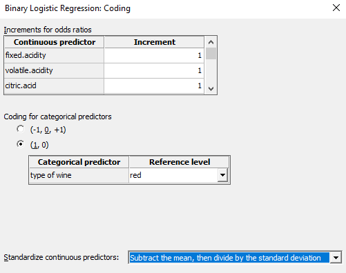
When introducing interactions, it is also useful to standardize the continuous predictors in your model to avoid, disturbing, scale effects (Stat > Regression > Regression > Fit Regression Model > Coding)
We used the stepwise method to automatically build the best model step-by-step and identify a useful subset of the terms out of a very large number of candidate terms. For that go to: Stat > Regression > Binary Logistic Regression > Fit Binary Logistic Model > Stepwise
The criteria that was used to identify the best model based on this stepwise approach was the Akaike Information Criteria (AIC). AIC estimates the relative amount of information lost by a given model, this statistic is used to compare different models. The smaller the AIC is, the better the model fits the data. AIC includes a penalty that increases with the number of estimated parameters to discourage overfitting. The objective is to avoid overfitting but also underfitting.
Ultimately, this iterative process leads us to the model below.
The Factors Contributing to Good-Tasting Wine
With 12 terms, this model might seem difficult to understand and explain, but it does give us a clue to how we can delve deeper into these data to better understand which factors contribute most to good-tasting wine.
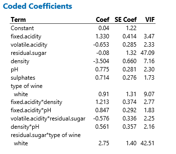
Coded (standardized) coefficients are useful to understand which variables are the most important:
Density has the largest effect (-3.504) then Residual Sugar coupled with Types of Wines (2.75 for the Residual Sugar * Types of Wines interaction ) has the second largest effect, then comes Fixed acidity (1.33) and the Fixed acidity * Density interaction (1.213)
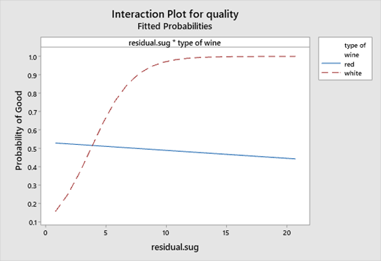
The interaction diagram above shows that the effect of Residual Sugar on wine quality, is virtually non existent in red wines, however it plays an important role in white wines.
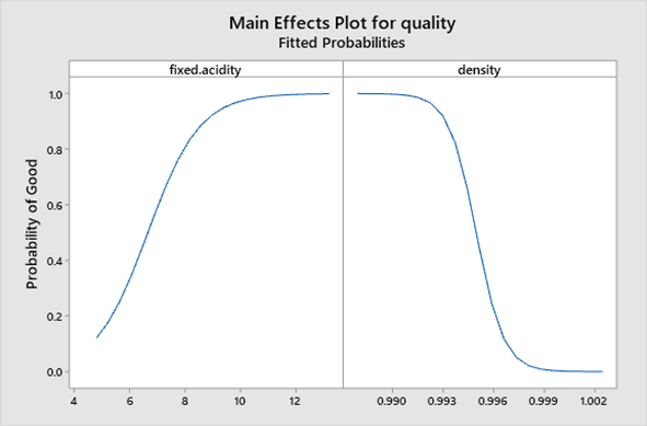
Now that we have models for the wines, we can see what the data tell us about the wine characteristics that influenced our panel’s rankings. For example, this main effects plot summarizes the relationship between fixed acidity, Density and the probability of making a good wine. Higher fixed acidity and a lower density tend to improve wine quality.
Conclusion
So when you need to understand situations that, at least on the surface, defy data analysis or when the number of candidate variables is large, why not dig a little deeper by using techniques such as binary logistic regression?
You can use a similar approach to what we did with this wine-tasting data to analyze marketing or sales data, to better understand customer preferences, and to gain insight into factors that are important—even if, like taste preferences, they seem hard to measure.
As a conclusion, we have been able to identify the best model thanks to a new feature of Minitab 19 -the stepwise approach based on the Akaike Information Criteria (AIC).
NEXT:
View our free webinar to learn "What's New in Minitab 19"
Discover the powerful new features of Minitab 19 that provide you with better decision making, faster performance and easier navigation. Click below to view the webinar and receive the recording: